Download Excel 2016: Core Data Analysis, Manipulation, and Presentation.77-727.ActualTests.2019-05-18.11q.tqb
| Vendor: | Microsoft |
| Exam Code: | 77-727 |
| Exam Name: | Excel 2016: Core Data Analysis, Manipulation, and Presentation |
| Date: | May 18, 2019 |
| File Size: | 5 MB |
How to open TQB files?
Files with TQB (Taurus Question Bank) extension can be opened by Taurus Exam Studio.
Purchase
Coupon: TAURUSSIM_20OFF
Discount: 20%
Demo Questions
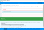
Question 1
Project 3 of 7: Tree Inventory
Overview
You are updating the inventory worksheet for a local tree farm.
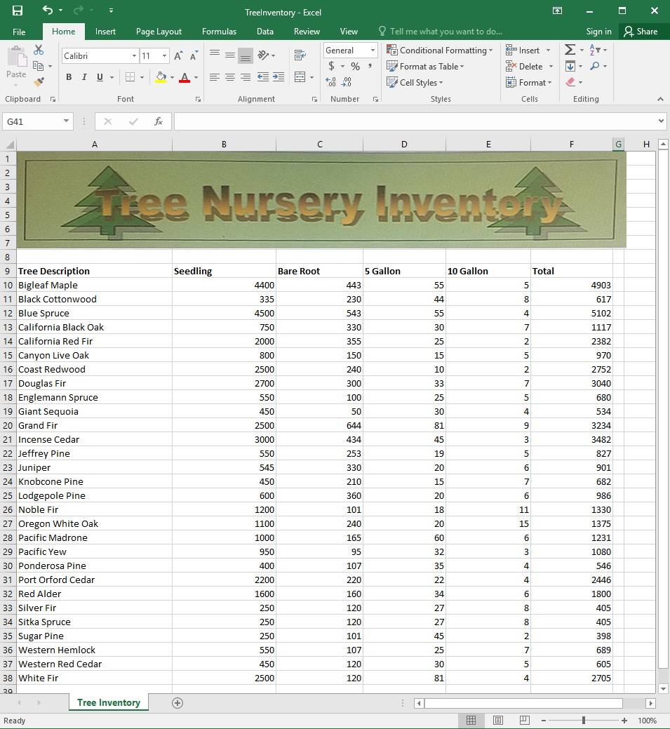
Check the spreadsheet for accessibility problems. Correct the error by adding “Tree Nursery Inventory” as an alternative text file. You do not need to fix the warning.
- See explanation below.
Correct answer: 1
Explanation:
1. To check the accessibility select the Review tab from the ribbon. 2. Select Check Accessibility. 3. Review the results. 4. Exit the Accessibility Checker. 5. Right-click on the worksheet then click Format and then click Alt Text. 6. Type “Tree Nursery Inventory” in the Description box. 7. Click OK. References:https://support.office.com/en-us/article/Use-the-Accessibility-Checker-to-find-accessibility-issues-a16f6de0-2f39-4a2b-8bd8-5ad801426c7f 1. To check the accessibility select the Review tab from the ribbon.
2. Select Check Accessibility.
3. Review the results.
4. Exit the Accessibility Checker.
5. Right-click on the worksheet then click Format and then click Alt Text.
6. Type “Tree Nursery Inventory” in the Description box.
7. Click OK.
References:
https://support.office.com/en-us/article/Use-the-Accessibility-Checker-to-find-accessibility-issues-a16f6de0-2f39-4a2b-8bd8-5ad801426c7f
Question 2
Project 4 of 7: Car Inventory
Overview
You manage the office of a used car business. You have been asked to prepare the inventory list for a big annual sale.
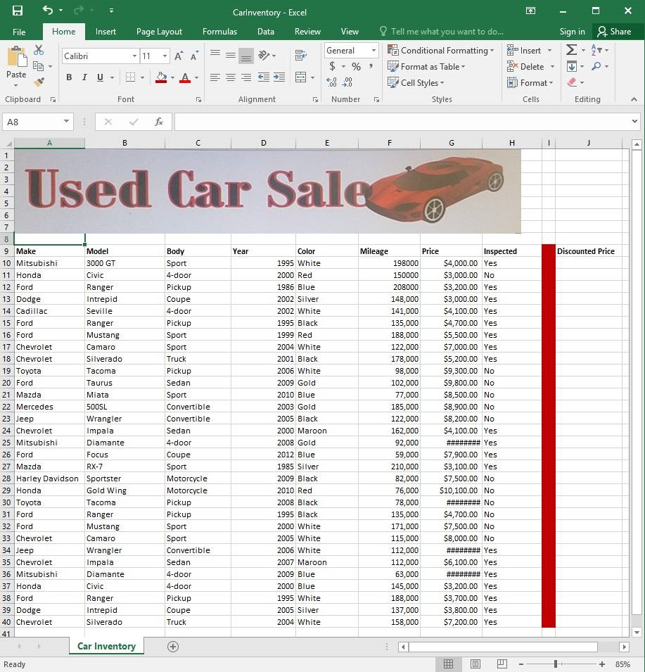
Configure the “Car Inventory” worksheet so the column headings in row 9 appear on all printed pages.
- See explanation below.
Correct answer: 1
Explanation:
1. On the “Car Inventory” worksheet, click Print Titles from the Page Setup group, situated on the Page Layout tab. 2. Under Print Titles, on the Sheet tab, type the reference of the row you want to reappear (row 9) in the Rows to repeat at top box. References:https://support.office.com/en-us/article/Print-rows-with-column-headers-on-top-of-every-page-D3550133-F6A1-4C72-AD70-5309A2E8FE8C 1. On the “Car Inventory” worksheet, click Print Titles from the Page Setup group, situated on the Page Layout tab.
2. Under Print Titles, on the Sheet tab, type the reference of the row you want to reappear (row 9) in the Rows to repeat at top box.
References:
https://support.office.com/en-us/article/Print-rows-with-column-headers-on-top-of-every-page-D3550133-F6A1-4C72-AD70-5309A2E8FE8C
Question 3
Project 4 of 7: Car Inventory
Overview
You manage the office of a used car business. You have been asked to prepare the inventory list for a big annual sale.
Simultaneously replace all instances of the text “Pickup” with the text “Truck”.
- See explanation below.
Correct answer: 1
Explanation:
1. Click Find & Select from the Editing group situated on the Home tab. 2. Click Replace. 3. Type the text “Pickup” in the Fine what box. 4. Click Options to further define the search, specify the “Car Inventory” worksheet select Sheet in the Within box. 5. Type “Truck” in the Replace with box. 6. Click Find All, and then click Replace All. 7. Finalize by clicking OK. References:https://support.office.com/en-us/article/find-or-replace-text-and-numbers-on-a-worksheet-0e304ca5-ecef-4808-b90f-fdb42f892e90 1. Click Find & Select from the Editing group situated on the Home tab.
2. Click Replace.
3. Type the text “Pickup” in the Fine what box.
4. Click Options to further define the search, specify the “Car Inventory” worksheet select Sheet in the Within box.
5. Type “Truck” in the Replace with box.
6. Click Find All, and then click Replace All.
7. Finalize by clicking OK.
References:
https://support.office.com/en-us/article/find-or-replace-text-and-numbers-on-a-worksheet-0e304ca5-ecef-4808-b90f-fdb42f892e90
Question 4
Project 5 of 7: City Sports
Overview
The city events manager wants to analyze the enrollment changes over the past five years for various adult and youth sports programs. You have been tasked to prepare tables for the analysis.
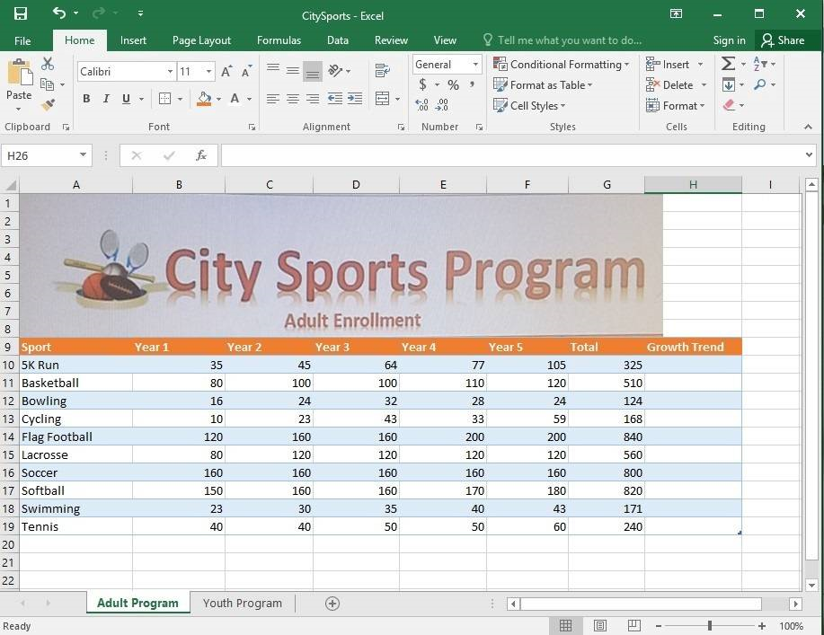
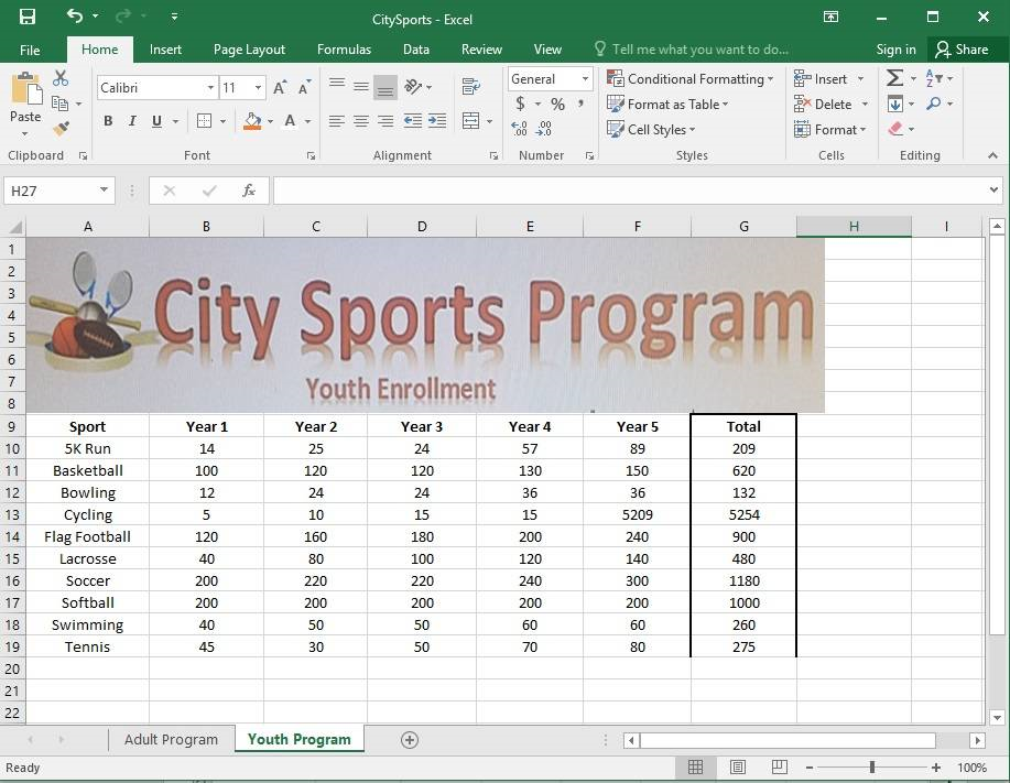
Add the Alternative Text Title “Adult Enrollment” to the “Adult_Program” table.
- See explanation below.
Correct answer: 1
Explanation:
1. Right-click the text title “Adult_Program” and click Format Object then click Alt Text. 2. Type “Adult Enrollment” in the Title box as desired. 3. Click OK. References:https://support.office.com/en-us/article/add-alternative-text-to-a-shape-picture-chart-smartart-graphic-or-other-object-44989b2a-903c-4d9a-b742-6a75b451c669#bkmk_o2016_2013 1. Right-click the text title “Adult_Program” and click Format Object then click Alt Text.
2. Type “Adult Enrollment” in the Title box as desired.
3. Click OK.
References:
https://support.office.com/en-us/article/add-alternative-text-to-a-shape-picture-chart-smartart-graphic-or-other-object-44989b2a-903c-4d9a-b742-6a75b451c669#bkmk_o2016_2013
Question 5
Project 6 of 7: Bike Tours
Overview
You are the owner of a small bicycle tour company summarizing trail rides that have been booked for the next six months.
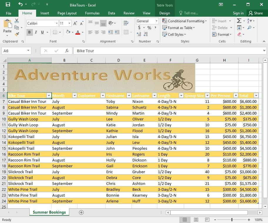
In cell M9 on the “Summer Bookings” worksheet, insert a function that calculates the number of groups containing 12 or more people even if the order of the rows is changed.
- See explanation below.
Correct answer: 1
Explanation:
1. In cell M9, on the “Summer Bookings” worksheet, insert the following COUNTIF formula: “=COUNTIF(G6:G24, >= 12”)”References:https://support.office.com/en-us/article/count-numbers-greater-than-or-less-than-a-number-453b0ccc-cfaa-4332-ad02-6e148e01aa0a 1. In cell M9, on the “Summer Bookings” worksheet, insert the following COUNTIF formula: “=COUNTIF(G6:G24, >= 12”)”
References:
https://support.office.com/en-us/article/count-numbers-greater-than-or-less-than-a-number-453b0ccc-cfaa-4332-ad02-6e148e01aa0a
Question 6
Project 6 of 7: Bike Tours
Overview
You are the owner of a small bicycle tour company summarizing trail rides that have been booked for the next six months.
In cell M10 on the “Summer Bookings” worksheet, insert a function that calculates the total amount of sales from the “Total” column for groups containing 12 or more people even if the order of the rows is changed.
- See explanation below.
Correct answer: 1
Explanation:
1. In cell M10 on the “Summer Bookings”, insert the following SUMIF formula: “=SUMIF(G6:G24, “>= 12”, I6:I24).”’References:https://support.office.com/en-us/article/SUMIF-function-169B8C99-C05C-4483-A712-1697A653039B 1. In cell M10 on the “Summer Bookings”, insert the following SUMIF formula: “=SUMIF(G6:G24, “>= 12”, I6:I24).”’
References:
https://support.office.com/en-us/article/SUMIF-function-169B8C99-C05C-4483-A712-1697A653039B
Question 7
Project 6 of 7: Bike Tours
Overview
You are the owner of a small bicycle tour company summarizing trail rides that have been booked for the next six months.
In cell C8 on the “Summer Bookings” worksheet, insert a function that joins the customer “Lastname” to the customer “Firstname” separated by a comma and space. (Example: Campbell, David).
- See explanation below.
Correct answer: 1
Explanation:
1. In cell C8 on the “Summer Bookings” worksheet, insert the following CONCAT function: “=CONCAT(E6 “, “D6)” OR “=E6& “, “, D6”.References:https://support.office.com/en-us/article/Combine-text-from-two-or-more-cells-into-one-cell-81ba0946-ce78-42ed-b3c3-21340eb164a6 1. In cell C8 on the “Summer Bookings” worksheet, insert the following CONCAT function: “=CONCAT(E6 “, “D6)” OR “=E6& “, “, D6”.
References:
https://support.office.com/en-us/article/Combine-text-from-two-or-more-cells-into-one-cell-81ba0946-ce78-42ed-b3c3-21340eb164a6
Question 8
Project 6 of 7: Bike Tours
Overview
You are the owner of a small bicycle tour company summarizing trail rides that have been booked for the next six months.
On the “Summer Bookings” worksheet, remove the table functionality from the table. Retain the cell formatting and location of the data.
- See explanation below.
Correct answer: 1
Explanation:
1. Click Design from the Ribbon on Table Tools. 2. In the Tools group, click on Convert to Range. OR 1. Right-click the table then click on Table then press Convert to Range. References:https://support.office.com/en-us/article/convert-an-excel-table-to-a-range-of-data-0b326ff1-1764-4ebe-84ea-786265d41c77?redirectSourcePath=%252fen-us%252farticle%252fRemove-a-table-without-losing-the-data-or-table-format-ADF88635-90F5-4FAA-9417-19862F38CCE8&ui=en-US&rs=en-US&ad=US 1. Click Design from the Ribbon on Table Tools.
2. In the Tools group, click on Convert to Range.
OR
1. Right-click the table then click on Table then press Convert to Range.
References:
https://support.office.com/en-us/article/convert-an-excel-table-to-a-range-of-data-0b326ff1-1764-4ebe-84ea-786265d41c77?redirectSourcePath=%252fen-us%252farticle%252fRemove-a-table-without-losing-the-data-or-table-format-ADF88635-90F5-4FAA-9417-19862F38CCE8&ui=en-US&rs=en-US&ad=US
Question 9
Project 6 of 7: Bike Tours
Overview
You are the owner of a small bicycle tour company summarizing trail rides that have been booked for the next six months.
Insert page numbering in the center of the footer on the “Summer Bookings” worksheet using the format Page 1 of ?.
- See explanation below.
Correct answer: 1
Explanation:
1. On the “Summer Bookings” worksheet, click Header & Footer from the Text group situation on the Insert tab. 2. Click Click to add footer which would display the Header & Footer tools which gets added to the Design tab. 3. Specify where the page number should be by selecting the Center section box. 4. On the Design tab in the Header & Footer Elements group, click Page Number. 5. The placeholder &[Page] will appear in the selected section, to add the total number of pages type the word of followed by the space in the Header & Footer Elements group after clicking Number of Pages, then the placeholder &[Page] of &[Pages] appear. 6. Click anywhere outside the header or footer area to display the page numbers in Page Layout View. 7. Once you are done working in the Page Layout View, click Normal in the Workbook Views group situated on the View tab. OR You can also click Normal on the status bar. References:https://support.office.com/en-us/article/Insert-page-numbers-on-worksheets-27A88FB9-F54E-4AC4-84D7-BF957C6CE29C 1. On the “Summer Bookings” worksheet, click Header & Footer from the Text group situation on the Insert tab.
2. Click Click to add footer which would display the Header & Footer tools which gets added to the Design tab.
3. Specify where the page number should be by selecting the Center section box.
4. On the Design tab in the Header & Footer Elements group, click Page Number.
5. The placeholder &[Page] will appear in the selected section, to add the total number of pages type the word of followed by the space in the Header & Footer Elements group after clicking Number of Pages, then the placeholder &[Page] of &[Pages] appear.
6. Click anywhere outside the header or footer area to display the page numbers in Page Layout View.
7. Once you are done working in the Page Layout View, click Normal in the Workbook Views group situated on the View tab. OR You can also click Normal on the status bar.
References:
https://support.office.com/en-us/article/Insert-page-numbers-on-worksheets-27A88FB9-F54E-4AC4-84D7-BF957C6CE29C
Question 10
Project 7 of 7: Farmers Market
Overview
You are the Director of a local farmers’ market. You are creating and modifying charts for a report which shows the amounts and variety of products sold during the season.
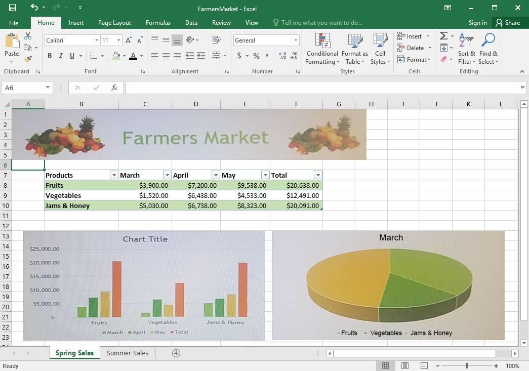
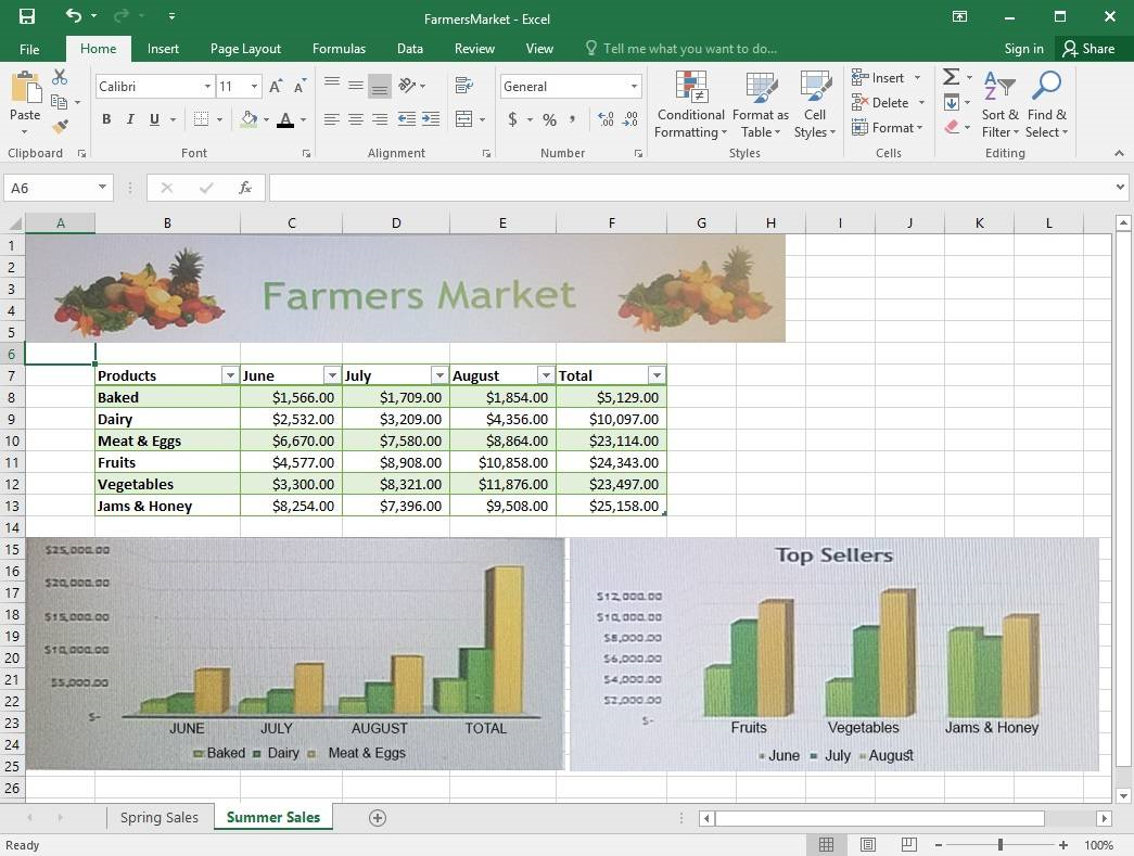
On the “Summer Sales” worksheet, use the data in the “Products” and “Total” columns only to create a 3-D Pie chart. Position the new chart to the right of the column charts.
- See explanation below.
Correct answer: 1
Explanation:
1. Select the data you would like to use, in this case it would be the data in the “Products” and “Total” columns from the “Summer Sales” worksheet. 2. Click on Insert Pie Chart situation on the Insert tab then pick the 3-D Pie chart as desired. 3. Format the chart as desired by using Chart Elements, the Chart Styles, or the Chart Filters. 4. Drag the Pie Chart to the desired location which is to the right of the column charts. References:https://support.office.com/en-us/article/Add-a-pie-chart-1A5F08AE-BA40-46F2-9ED0-FF84873B7863 1. Select the data you would like to use, in this case it would be the data in the “Products” and “Total” columns from the “Summer Sales” worksheet.
2. Click on Insert Pie Chart situation on the Insert tab then pick the 3-D Pie chart as desired.
3. Format the chart as desired by using Chart Elements, the Chart Styles, or the Chart Filters.
4. Drag the Pie Chart to the desired location which is to the right of the column charts.
References:
https://support.office.com/en-us/article/Add-a-pie-chart-1A5F08AE-BA40-46F2-9ED0-FF84873B7863
HOW TO OPEN VCE FILES
Use VCE Exam Simulator to open VCE files
HOW TO OPEN VCEX FILES
Use ProfExam Simulator to open VCEX files
ProfExam at a 20% markdown
You have the opportunity to purchase ProfExam at a 20% reduced price
Get Now!